Article
Abstract
Urban heat screening indices combine land surface temperature, vegetation, population and access to cooling space, but their maps depend on inclusion and weighting choices. We examine how spatial priorities change across four screening models in the five mainland administrative cities of Jakarta, Indonesia, on a 500 m grid (2,536 common cells). M1 ranks land surface temperature; M2 adds vegetation; M3 adds modelled total population; and M4 adds a count of children and older adults plus walking-network distance to 1,015 OpenStreetMap candidate parks. Thermal and demographic inputs refer to a declared 2024 period; the park and network snapshot is from November 2026. The M1 and M4 top deciles share 141 of 254 cells (55.5% retention; Jaccard 0.384). Between M3 and M4, a three-factor decomposition attributes 85.5% of absolute rank movement to park addition, 13.2% to reweighting and 1.3% to the age-count substitution. The age count is nearly collinear with population (Spearman ): replacing it with total population leaves the top decile almost unchanged (Jaccard 0.977), whereas an age-share specification changes it substantially (0.347). Under the additive M4, the top-decile cutoff (0.8737) exceeds the maximum score of all 537 near-park cells (0.8696), so no cell within 500 m of a candidate park enters the top 254; this is a property of the index and observed inputs, not evidence that parks are unimportant. The 229 excluded cells are cooler, greener and more peripheral than included cells, so the results describe a conditional sample rather than all of Jakarta. The study is an exploratory attribution and uncertainty analysis, not a validated health-risk or public-access model.
Keywords urban heat · land surface temperature · spatial prioritization · park accessibility · composite indicators · sensitivity analysis · spatial inequality · Jakarta
1Introduction
Urban heat is a planning problem before it is a measurement problem. Cities must decide where to plant trees, open cooling spaces, retrofit buildings or target public health outreach, and these decisions require some ordering of places. Satellite land surface temperature (LST) is attractive for that task because it is spatially continuous, repeatable and available at metropolitan scale (1, 2). LST has therefore become a common first layer in urban heat assessments, including in Jakarta (3–5). Yet LST is a surface property retrieved from clear-sky remote sensing; it is not air temperature, personal heat exposure or a health outcome (2, 6). A map of the hottest pixels is a map of one hazard component, not a map of where people are most exposed or where an intervention would do the most good.
Planning questions usually require more than a hazard layer. Exposure asks how many people are present; vulnerability asks whether some groups face greater risk for a given exposure; and accessibility asks whether people can reach cooling or green space (7–9). These are distinct constructs. Combining them into a single composite index is a legitimate decision-support strategy, but the combination is not a neutral act: it encodes a theory of what matters, a set of weights, a normalisation rule and a definition of access (10–12). Two indices can use the same data and produce different priority maps because they answer different questions. The policy relevance of a composite therefore depends on how transparently those choices are exposed and how strongly the resulting ranking depends on them.
Jakarta provides a demanding setting for this problem. The metropolitan region is hot, humid and highly unequal in built form and green-space provision. LST and vegetation studies document strong intra-urban thermal contrasts (3–5), while demographic and epidemiological work shows that older adults face elevated heat-related mortality risk (13). Heat is also experienced through social practice and everyday access to shade, water and communal space, particularly in informal settlements (14). Park access is uneven and cannot be inferred from park counts alone; it depends on the pedestrian network, entrances, permissions and the quality of destinations (15–17). Jakarta therefore offers a case where a heat-only map is clearly incomplete, but where the information needed to complete it is itself uncertain.
A growing literature combines heat, demographic vulnerability and green-space access. Jakarta studies include long-term urban heat island mapping (18), regression-informed vegetation adaptation priorities (19), and child-specific green-space vulnerability (20). Elsewhere, accessibility-based thermal assessments combine cooling supply, heat exposure and network catchments (21, 22), while composite heat-risk indices aggregate UHI intensity, green cover and population density into planning tiers (23), and reviews of green-infrastructure siting synthesise the indicator choices behind these rankings (24). A parallel literature asks whether priority rankings survive alternative aggregation choices, including weight and threshold scenarios in Jakarta (19) and equal-weight versus principal-component indices in Taiwan (25). These studies establish the relevance of the components and the value of sensitivity testing. They leave less examined the attribution of a sequential model transition: how much of a ranking change follows from adding a construct rather than from reweighting, and how candidate-park and pedestrian-network uncertainty propagates into the resulting priorities in Jakarta. Those questions are methodological and empirical at once, and they are the focus of this study.
We ask four questions. First, how much do priority rankings and top-decile sets change when LST is supplemented with vegetation, population, age count and modelled park distance? Second, what share of the M3-to-M4 change is attributable to park addition, reweighting and the age substitution? Third, how sensitive are the priorities to plausible assumptions about park destinations, connector permissions, missing routes and demographic specification? Fourth, how do sample eligibility and local spatial-inference conventions limit what can be inferred from the resulting map? We answer these questions using a reproducible 500 m grid analysis of the five mainland cities, built from processed thermal, demographic and accessibility layers (26).
Our analysis does three things. It quantifies how top-decile membership and rank positions change across the four specifications and how much of the M3-to-M4 change is attributable to park addition, reweighting and the age substitution. It shows, for Jakarta, that an age-count term adds little information beyond total population while an age-share specification changes the objective and the geography, and that an additive park-deficit term can determine the top decile under the observed inputs. It then uses those results as a cautionary case: a park term can dominate a ranking without demonstrating that parks are unimportant, that public access is unequal, or that M4 is a better model than M1–M3. The contribution is therefore an attribution and uncertainty analysis of a screening index, not a validated vulnerability model or a health-impact study.
Section 2 situates the work in prior literature. Section 3 describes the study area and data. Section 4 gives the complete methodology. Section 5 reports results, Section 6 discusses their interpretation, and Section 7 states limitations. Section 8 concludes. Supplementary material contains additional sensitivity tables, a data-quality register and figure provenance.
2Related Work
2.1Land surface temperature and the urban heat island
The urban heat island is a well-established phenomenon in which built surfaces and reduced vegetation alter the surface energy balance (1). Thermal remote sensing makes the surface expression of that balance observable at fine spatial resolution (2). LST is strongly related to vegetation abundance: greener and more vegetated surfaces tend to be cooler, and the LST–NDVI relationship has been used widely to map surface urban heat islands (27–29). Satellite platforms also reveal that surface urban heat island intensity varies substantially across cities and regions (28, 30). These studies justify LST and NDVI as screening layers. They also caution against equating LST with air temperature or human heat stress; the relationship between surface and air temperature is context-dependent (6). Our M1 and M2 models are deliberately simple representations of this tradition.
2.2Exposure, vulnerability and composite indices
Heat vulnerability indices combine hazard with demographic sensitivity and adaptive capacity. Reid et al. (7) mapped community determinants of heat vulnerability in the United States, and Wolf and McGregor (8) developed a heat-wave vulnerability index for London. Such indices are useful for communication and screening, but they are sensitive to indicator selection, weighting, normalisation and aggregation (11, 12, 31). A composite can change rankings even when the underlying data are unchanged. This is not a defect unique to heat indices; it is a general property of multidimensional indicators. Elmarakby and Elkadi (23) illustrate the planning use of this logic in a district Heat Risk Index that combines UHI intensity, green cover and population density, while Perdinan et al. (19) build a regression-informed vegetation-adaptation priority index for Jakarta. Such indices make priorities legible, but the index itself does not show how much a ranking change follows from adding a construct rather than from reweighting.
A parallel literature examines inequality in heat exposure. Chakraborty et al. (32) found disproportionately higher exposure to urban heat in lower-income neighbourhoods across multiple cities; Hsu et al. (33) documented unequal exposure to urban heat island intensity across major US cities; and Tuholske et al. (34) quantified global urban population exposure to extreme heat. Heat-health risk frameworks combine hazard, exposure and social vulnerability in related ways (35). These studies establish that exposure is uneven, but they generally do not model walking access to cooling destinations or decompose the effect of an access term on a priority ranking. Our work is closer to a screening and sensitivity exercise than to an epidemiological exposure assessment.
2.3Age, heat and green-space access
Children and older adults are often treated as heat-vulnerable groups. Reviews of temperature and mortality report elevated risk among older adults (36, 37), and children’s outdoor microclimates raise distinct physiological and behavioural concerns (38). Global projections suggest that heat exposure of older adults will increase substantially (39). In Jakarta, Varquez et al. (13) projected future increases in elderly heat-related mortality under urbanisation and climate change. These findings motivate an age-sensitive screening layer. They do not imply that an age count is a measure of vulnerability composition: counts largely track population size, whereas shares describe the relative presence of vulnerable groups.
Green-space access is similarly multidimensional. Reviews document inequities in park provision and quality (15, 16), and accessibility metrics differ in whether they measure distance, travel time, network reach or perceived access (17). GIS studies have long used network distance to assess park distribution (40); spatial-accessibility methods provide a broader family of distance, catchment and floating-catchment measures (41, 42), and walking-network studies make the route itself the object of analysis (43). More recent work incorporates cooling weights and older-adult demand (22). Feng et al. (44) analyse the distribution and accessibility of urban parks in Beijing, and Zhang et al. (45) examine park size thresholds, cooling accessibility and equity. Park cooling itself depends on size, vegetation, configuration and distance (46–49). Access to a cooling refuge is also an equity question in its own right (50, 51). Ramadhanis et al. (20) combine under-five population density with OSM green-space network distance in Jakarta, and Dong et al. (21) use an improved two-step floating catchment area and bivariate local Moran’s I to compare cooling accessibility with heat-risk exposure in Zhengzhou. These studies make accessibility the estimand. Our park term is a simpler candidate-park distance inside a composite screening index, and our contribution concerns the sensitivity of the resulting ranking rather than a new accessibility metric. The broader point is that a park-distance term is a model of access, not a measurement of public access. OSM completeness and tagging quality vary, and network routing depends on connectors and permissions that are rarely verified (52–54). Our treatment of candidate parks as a proxy, and our explicit stress tests, follow from this literature.
2.4Sensitivity, robustness and spatial inference
Composite-indicator research has developed a rich toolkit for uncertainty and sensitivity analysis (11, 12, 31). The central lesson is that rankings should be reported with the assumptions that generate them, not as unconditional facts. In parallel, spatial-analytic work provides global and local measures of autocorrelation (55, 56), but local inference is sensitive to the choice of weights, tail specification, permutation count and multiple-testing correction (57, 58). A cluster map is therefore not a self-interpreting result. Fitria et al. (25) make this explicit by comparing equal-weight and PCA heat-vulnerability indices across 158 Taiwanese districts and mapping where their priority rankings disagree; Perdinan et al. (19) test weight and threshold stability in Jakarta. Our design complements that work by attributing a sequential M3-to-M4 change to park addition, reweighting and age substitution, and by propagating candidate-park and network uncertainty through the ranking rather than treating the destination layer as fixed.
2.5Jakarta-specific evidence
Jakarta has a substantial applied literature on LST, vegetation and heat. Putra et al. (4) document increasing urban heat island area in relation to land-use change; Siswanto et al. (3) characterise the spatio-temporal urban heat island of the Jakarta metropolitan area; and Rizki et al. (5) examine the impact of urban green space on the heat island in East Jakarta. Ulfiasari and Yola (18) use Landsat 5 and 8 imagery to trace a decade of UHI expansion across the Jakarta metropolitan area; Perdinan et al. (19) develop regression-informed vegetation-adaptation priorities for Jakarta; and Ramadhanis et al. (20) assess child-specific green-space accessibility with WorldPop and OSM network data. Salsabila et al. (14) show through ethnographic and practice-based work that cooling in Jakarta’s informal settlements is entangled with social life and communal space, and Manik and Syaukat (59) compare heat vulnerability in two tropical Indonesian cities. These studies establish local relevance, multi-indicator prioritisation and green-space accessibility as active research questions. They leave less examined how a sequential change from heat-only to heat–population–age–park screening reshapes cell-level priorities, and how modelled candidate-park destinations and routing change that ranking.
2.6Positioning and contribution
Table 1 summarises the closest bodies of work. It is not a systematic review and does not establish that no similar study exists. Every individual ingredient of our analysis has precedent: LST–NDVI mapping, heat vulnerability indices, age-sensitive risk, network-based park access and composite-indicator sensitivity. Recent Jakarta work already combines thermal condition, vegetation deficit, built-up intensity and population exposure in an adaptation-prioritisation framework and tests weight and threshold stability (19); recent Taiwanese work treats disagreement between priority rankings as a decision-support diagnostic (25). Neither the combination itself nor sensitivity analysis is new. What remains is narrower: a cell-level attribution of a sequential screening transition, a test of age-count redundancy, and an uncertainty analysis of modelled candidate-park accessibility in Jakarta. We present that contribution as conditional on the analytical specification and the sensitivity analyses reported below.
| Study | Context / unit | Indicators / construct | Spatial method / uncertainty | Closest overlap | Evidence-backed distinction |
|---|---|---|---|---|---|
| Perdinan et al. (2026) | Jakarta; 30 m pixels, municipal aggregation | LST, vegetation deficit, built-up intensity, population density | OLS regression; weighted priority index; four weight scenarios and threshold relaxation | Jakarta multi-indicator adaptation prioritisation and stability testing | Regression-informed adaptation tiers, not our sequential screening models; no age count/share, candidate-park network uncertainty or Shapley decomposition |
| Fitria et al. (2026) | Taiwan; 158 districts | 17 exposure, sensitivity and adaptive-capacity indicators | Equal-weighting versus PCA; Spatial Disagreement Index; leave-one-out sensitivity | Explicit ranking disagreement and decision support | Disagreement between aggregation methods; we decompose a sequential construct transition and modelled candidate-park uncertainty |
| Ramadhanis et al. (2026) | Jakarta; fishnet grid | Under-five population density; OSM green-space distance | Network shortest path; child green-space vulnerability index | Jakarta children and green-space access | Age-specific vulnerability map; we compare age counts with shares in a multi-model ranking and use all-age candidate parks |
| Dong et al. (2024) | Zhengzhou; 2010, 2015 and 2020 | Urban green space, heat-island area, residents | Improved 2SFCA; bivariate local Moran’s | Cooling accessibility combined with heat-risk spatial statistics | Accessibility is the estimand; no M1–M4 composite ranking or attribution decomposition |
| Elmarakby & Elkadi (2024) | Manchester; districts | UHI intensity, green cover, population density | Heat Risk Index; correlation; planning tiers | Composite heat-risk prioritisation | District risk index, not cell-level screening; no age count/share or network uncertainty |
| Ulfiasari & Yola (2022) | Jakarta metropolitan area | Landsat UHI intensity and area over ten years | Remote-sensing change mapping; planning interpretation | Jakarta UHI mapping for spatial planning | Maps UHI distribution and trends; no multi-indicator priority ranking or rank-change analysis |
| Kim & Kwak (2026) | Older adults; walking network | Cooling-weighted park accessibility | Generalised two-step floating catchment area | Age and park-access measurement | Focus on the accessibility model rather than Jakarta ranking sensitivity or count/share redundancy |
| This study | Five mainland Jakarta cities; 500 m grid | LST, vegetation, population, age count/share, candidate-park distance | M1–M4; Jaccard; Shapley; 52 scenarios; LISA | Attribution, demographic redundancy and candidate-park uncertainty | Conditional screening analysis; not a validated risk, health or public-access model |
LST: land surface temperature; UHI: urban heat island; 2SFCA: two-step floating catchment area; PCA: principal component analysis. The table summarises the research question and evidence used in each study; it does not claim to reproduce every method. The absence of a study is not evidence that no similar work exists.
3Study Area and Data
3.1Study area and spatial unit
The study covers the five mainland administrative cities of Jakarta, Indonesia: West Jakarta (Jakarta Barat), Central Jakarta (Jakarta Pusat), South Jakarta (Jakarta Selatan), East Jakarta (Jakarta Timur) and North Jakarta (Jakarta Utara). Kepulauan Seribu, the offshore administrative regency, is excluded. The analysis unit is a 500 m lattice in the projected UTM zone 48S coordinate reference system (EPSG:32748), clipped to the five-city land boundary. The master grid contains 2,765 cells. Because the lattice is clipped to a complex coastline and administrative boundary, 383 cells are partial polygons; 65 have less than 10% of the nominal 0.25 km area, and the smallest is approximately km. These slivers are retained and flagged rather than silently deleted, because deleting them would change the population accounting and the spatial graph.
The grid is a spatial sampling device, not a cadastral or neighbourhood unit. Cell-level results are therefore subject to the modifiable areal unit problem: different partitions of the same land could produce different rankings and different local statistics (60). We do not treat the 500 m cell as a meaningful social unit. It is a common, reproducible support on which heterogeneous raster and vector inputs can be compared.
3.2Thermal and vegetation data
LST and NDVI were derived from Landsat 9 Collection 2 Level-2 surface reflectance and surface temperature products (dataset LANDSAT/LC09/C02/T1_L2) (61) for a declared 2024 window (1 January to 31 December 2024). The intended recipe filters to L2SP products, masks fill, dilated cloud, cirrus, cloud, cloud shadow and snow using QA_PIXEL bits 0–5, requires QA_RADSAT = 0, converts ST_B10 to Celsius using the Collection 2 scale factors, computes NDVI from SR_B4 (red) and SR_B5 (near-infrared), and takes a per-pixel median composite across clear observations. Each band is reduced independently, so the LST and NDVI medians for a pixel may derive from different acquisition dates. The composite is exported at 30 m in EPSG:32748.
Dynamic World class probabilities are available for 2,764 cells (62), but categorical class fractions were not exported; M1–M4 do not use them, and we make no categorical land-cover claim. Grid values are area-weighted means over valid pixels within each clipped cell, computed with exactextract. A cell is flagged for low thermal support when the valid LST area fraction is below 0.50; this is a quality-control choice for the analysis. One cell (JKT_R037_C062) has 27.759% valid LST area (6,724.1 m of 24,223.1 m) and is excluded from all models under the 0.50 rule. The delivered LST and NDVI values for that cell are retained in the source table, but the cell does not enter the common comparison sample. We do not interpret low-support cells as having no heat.
The critical provenance limitation is that the original Earth Engine scene, task and AOI records could not be recovered. The scene manifest is header-only; this means that records are unavailable, not that zero scenes were acquired. The 2024 label is therefore a declared recipe period, not an independently verified acquisition history. Annual clear-observation counts are available, but monthly and seasonal sampling cannot be reconstructed from the median raster alone. We make no claim of seasonal representativeness, annual mean temperature, temporal trend or a verified 2024 snapshot.
3.3Population and age data
Population inputs are from the WorldPop Global2 R2025A release, which provides modelled people per grid cell at approximately 100 m (3 arc-second) resolution for a 2024 reference year, including total population and age/sex groupings (63). We use total population, children aged 0–14 and older adults aged 65 and over. These are modelled estimates, not a census or a register. They describe residential population, not daytime presence, mobility or personal exposure.
Zonal aggregation uses the project’s hybrid rule: where more than one valid source-pixel centre falls inside a clipped cell, the valid centre values are summed; otherwise, intersecting valid pixels are allocated fractionally by their intersection area. A fractional alternative allocates every valid native pixel by its polygon intersection fraction and is additive under changes of partition. The hybrid rule is not additive under repartitioning because centres may be selected differently in each polygon. The primary analysis uses the hybrid rule for continuity with the baseline configuration; the fractional alternative is a sensitivity scenario. Population counts are never multiplied by coverage a second time.
Source support is treated explicitly. Of 19 cells that originally had no valid age-raster support, 13 were recovered by retrieving buffered age surfaces that cover the five-city union with a 1,000 m buffer. Six cells remain unsupported in total population and both age groups: JKT_R003_C031, JKT_R057_C063, JKT_R061_C009, JKT_R061_C010, JKT_R061_C011 and JKT_R062_C043. They are retained in the master grid with analytical nulls, while their original exported zeros are preserved in *_raw columns. A null is not a estimated population of zero. Two of the six unsupported cells are substantively large (JKT_R061_C009: 0.244 km, 97.8% coverage; JKT_R061_C010: 0.099 km, 39.5% coverage), both in North Jakarta.
3.4Candidate parks and the pedestrian network
Park destinations are derived from an OpenStreetMap snapshot extracted on 19 November 2026. The inventory contains 1,015 candidate park polygons. Each candidate was reviewed against archived OSM tags and, where available, official or operator context. No candidate has verified public access and no candidate has a verified physical entrance: 980 are classified as unknown, 28 as conditional and unverified, and 7 as carrying a positive OSM access tag that remains unverified. All 1,015 are unresolved in the evidence register. A positive OSM tag is an assertion, not a field verification; an unknown tag is not evidence of closure. The candidate set is therefore a destination proxy, not a public-park inventory. Table 2 summarises the evidence states.
Walking distances were computed on a pedestrian graph built from the same OSM snapshot. Each grid cell and each candidate park is connected to the graph at a nearest node; the park is represented by a representative point inside its polygon, not by a verified entrance. The baseline distance is the shortest-path network distance to any non-restricted candidate park, capped at 1,000 m for the park-deficit term. The cap is a modelling choice, not a measured threshold of park utility. Of 2,765 master cells, 226 have no route to a candidate park in the baseline graph. These are retained as missing and excluded from the common comparison sample; they are not assigned a distance of zero, infinity or the cap.
Two route-permission stress scenarios are used. A conservative scenario removes edges incident on, or matching, explicitly forbidden source nodes (foot=no/private, or access=no/private without an explicit permissive foot override) and excludes direct connectors that touch those nodes. It removes 24,370 directed edges and increases missing routes from 226 to 407. A positive-tag-only destination scenario retains only destinations with a positive access or permissive tag; it contains 10 destinations (9 tagged yes and 1 permissive), of which 8 are within 500 m and 41 within 1,000 m of a routable origin; 2,482 cells are saturated at the 1,000 m cap. This scenario is a coverage stress test, not a better estimate of access. In the connector audit, 167 origin connectors and 78 park connectors conflict with explicit OSM node restrictions. These conflicts are retained in the evidence file and are not silently repaired.
| Evidence state | Candidates | Share |
|---|---|---|
| Unknown access | 980 | 96.55% |
| Conditional, unverified | 28 | 2.76% |
| Positive OSM tag, unverified | 7 | 0.69% |
| Verified public access | 0 | 0.00% |
| Verified physical entrance | 0 | 0.00% |
| Unresolved review status | 1,015 | 100.00% |
Evidence states are hierarchical and are not simple access-tag counts. A positive OSM tag is an unverified assertion; an unknown tag is not evidence of closure. The positive-tag-only scenario retains 10 destinations and is a coverage stress test, not a better estimate of public access.
3.5Reference periods and source table
The analysis mixes reference periods. LST and NDVI refer to the declared 2024 thermal period; WorldPop refers to a 2024 reference year; and the park and pedestrian network is a 19 November 2026 snapshot. We do not have a historical OSM archive: six requests for historical snapshots failed, and no temporal comparison is possible. The resulting object is a mixed-period candidate proxy. It can support statements about how a 2024 thermal/demographic pattern combines with a 2026 candidate-access network under explicit assumptions. It cannot support statements about 2024 public access, seasonal heat exposure, temporal change or the effects of a 2026 network on 2024 residents. Table 3 summarises the sources, their processing and their main limitations.
| Dataset | Variable | Reference period | Native resolution | Processing | Main limitation |
|---|---|---|---|---|---|
| Landsat 9 Collection 2 Level-2 (USGS) | LST, NDVI, thermal QA | 2024 (declared) | 30 m | Clear-sky per-pixel median composite; QA_PIXEL bits 0–5 and QA_RADSAT; area-weighted zonal mean | Scene/task/AOI lineage unavailable (RS-01); surface not air temperature; seasonal representativeness unverified |
| WorldPop Global2 R2025A | Total population; ages 0–14 and 65+ | 2024 reference year | 100 m (3 arc-second) | Modelled people per cell; hybrid or fractional zonal allocation | Model estimates, not census; 6 cells without age support; 383 partial cells |
| OpenStreetMap (OSM) | Candidate park polygons | 2026-11-19 snapshot | Vector | 1,015 candidates; representative point; nearest graph node | 0 verified public access or entrances; 980 unknown; 1,015 unresolved |
| OSM pedestrian network | Walking graph | 2026-11-19 snapshot | Vector | Shortest path; 1,000 m cap; baseline 226 missing routes | Modelled, unvalidated routes; 167 origin and 78 park connector conflicts; 407 missing under conservative policy |
| Administrative boundaries | Five mainland city polygons | Study definition | Vector | 500 m UTM lattice clipped to land | Kepulauan Seribu excluded; boundary vintage not independently audited |
| Analysis grid | 500 m cells | Study definition | 500 m | 2,765 cells in EPSG:32748 | 383 partial cells; 65 cells below 10% nominal area |
LST: land surface temperature; NDVI: Normalized Difference Vegetation Index; QA: quality assurance; AOI: area of interest. The 2024 label is a declared recipe period, not an independently verified acquisition history. Park distance is a modelled network proxy, not measured public access.
4Methods
4.1Sample eligibility and the common comparison set
All models are compared on a common set of cells for which every required input is available. This avoids the common error of comparing correlations or top-set overlap across different sample sizes. Starting from 2,765 master cells, 229 are excluded: 222 have a missing walking route only; 4 have missing route, population and age support; 2 have missing total population and age support but a known route; and 1 has low LST support under the 50% valid-pixel rule. The union is 229, because the route-missing and support-missing categories overlap. The common set is therefore 2,536 cells (91.7%; Table 4). Model-specific eligibility is 2,764 for M1 and M2, 2,758 for M3 and 2,536 for M4. M1 and M2 differ from the master grid only by the low-LST cell; M3 additionally loses six cells without population support; M4 additionally loses the route-missing and age-unsupported cells.
The common set is not a random sample of Jakarta. The excluded cells are systematically cooler, greener, more peripheral and less connected than the included cells. We report their profile in Section 5.8 and treat the common-set result as a conditional estimand. For spatial statistics, one additional cell (JKT_R013_C019) is a Queen-contiguity island; it is removed from the graph, leaving 2,535 observations and 18,368 directed edges. This island is a graph property, not a source-support exclusion.
| Category | Cells | Note |
|---|---|---|
| Master grid | 2,765 | Five mainland cities; 500 m lattice |
| M1 / M2 eligible | 2,764 | Excludes one low-LST-support cell (JKT_R037_C062) |
| M3 eligible | 2,758 | Also excludes six cells without population support |
| M4 eligible (common set) | 2,536 | Also excludes age-unsupported and route-missing cells |
| Excluded from common set | 229 | 8.28% of master grid |
| Route missing only | 222 | No path to a candidate park in baseline graph |
| Route + population + age missing | 4 | Already outside common set because of route |
| Population/age missing only | 2 | JKT_R003_C031, JKT_R057_C063 |
| Low LST support | 1 | JKT_R037_C062; 27.759% valid LST area |
| Spatial observations after island removal | 2,535 | JKT_R013_C019 is a Queen island |
The two population-only exclusions explain the difference between the 2,538-cell benchmark and the 2,536-cell common set. They are slivers (0.000266 and 0.002643 km) with no source support; their original exported zeros are preserved as raw values, not treated as estimated population.
4.2Zonal aggregation and normalisation
For a cell and a variable , let be the area-weighted mean over valid source pixels, or the modelled population count allocated to the cell. Each model component is normalised to using a percentile-clipped min–max rule computed on the common sample:
where and are the 5th and 95th percentiles of the component in the common sample. Values below the 5th percentile are set to zero and values above the 95th percentile to one. The rule reduces the influence of extreme cells and makes components comparable, but it also saturates scores: M1 has 127 cells tied at the maximum. Ties are broken deterministically by the unclipped min–max score and then by grid identifier, so the ranking does not depend on row order. The park-deficit component is not renormalised after capping; it is defined directly on a 0–1 scale as , where is the modelled network distance in metres.
4.3The four screening models
The four models are nested in data requirements but not in statistical estimation. They are alternative constructs, not successive estimates of one latent quantity. Let be LST, NDVI, total population, the population aged 0–14, the population aged 65 and over, and the candidate-park network distance. The scores are
M1 is a heat-only screening model. M2 adds a vegetation-deficit term. M3 adds total population exposure. M4 replaces total population with a count of children and older adults and adds the park-deficit term. The weights are a modelling choice: they were fixed before the real LST data were available and are not derived from a Jakarta-specific literature. They are therefore reported as a configuration, not as a validated standard. The model formulas are reproduced exactly from model_specification.json; M4 is not redefined in this paper.
Table 5 summarises the four score definitions. M4 is best described as an exploratory heat–population–park-deficit screening index. It is not an age-vulnerability model and not a health-risk model. The age term is a count, not a share. Because children and older adults are a nearly constant fraction of the modelled population in this dataset, the count term is almost collinear with total population. A separate age-share scenario is used to show what a composition-oriented question would look like; it is not the primary M4 specification.
| Model | Score definition | Question addressed |
|---|---|---|
| M1 | Where is the surface hottest? | |
| M2 | Where is heat combined with low vegetation? | |
| M3 | Where do heat, low vegetation and many residents coincide? | |
| M4 | Where does the heat–population–park-deficit screening rule score high? |
M4 is an exposure-oriented screening index, not an age-composition model, a health-risk model or a causal model. The age term is a count. The park term is a modelled network proxy to candidate destinations with unverified public access and entrances.
4.4Ranking, top-priority sets and model comparison
Cells are ranked in descending score, with rank 1 assigned to the highest score. The top-priority budget is cells, i.e. the top decile. We also report 5% (127 cells) and 20% (508 cells) budgets to show threshold dependence. Two models are compared using Spearman’s rank correlation, Kendall’s , the Jaccard overlap of their top- sets, and the mean and median absolute rank shift. For top sets and ,
Jaccard is 0 for disjoint sets and 1 for identical sets. It is sensitive to the budget: a small top set can have low overlap even when the underlying scores are highly correlated. We therefore report Jaccard at three budgets (Table 6) and never treat a single value as a general measure of model agreement.
4.5Attribution of M3-to-M4 change
The M3-to-M4 difference combines three changes: the addition of a park-deficit term, the reweighting of the shared LST and NDVI terms, and the substitution of the age count for total population. Let the score change be
The three terms sum exactly to the score difference. To attribute rank movement rather than score movement, we compute the exact three-factor Shapley value of the induced ranking over all coalitions. For each cell, the marginal rank gain of adding a factor is evaluated in every order, and the average is taken. The absolute Shapley contributions are then normalised to sum to 100%. This is a descriptive decomposition of a model change, not a causal effect of parks, age or weights on real-world outcomes.
We also run matched-weight ablations that hold the sample and normalisation anchors fixed. These include M3, a reweighting-only variant, an age-swap-only variant, a park-addition-only variant, all pairwise combinations, the full M4, a no-park variant, a park-only variant, a heat-only variant, an equal-weight variant, a total-count swap, a vulnerable-share variant, child-share and elderly-share variants, and a proportional M3-plus-park variant. These ablations answer different questions and are not all equally plausible policy alternatives; Tables 7 and 8 report the main results and state their baselines explicitly.
4.6Park-access and demographic sensitivity scenarios
Park-access uncertainty is evaluated with four families. First, destination scenarios vary the candidate set: baseline, positive-tag-only, and alternative nearest-distinct-park assignments. Second, permission scenarios vary the graph: baseline, conservative node/connector removal, and a positive-tag stress variant. Third, missing-route scenarios assign no distance (baseline exclusion), the observed median distance, or the 1,000 m cap; these bound the effect of unknown routes but are not estimates of true access. Fourth, distance-cap scenarios vary the cap (750, 1,000 and 1,500 m) and the park threshold (500 and 1,000 m). For each scenario we recompute normalisation on the scenario’s eligible set and report Jaccard against the baseline M4 top decile. We distinguish an eligibility-changing comparison, in which the sample changes, from a fixed-anchor comparison, in which the same cells and normalisation anchors are used. The latter isolates rank changes from sample changes. The resulting family envelope is reported in Section 5.10.
Demographic sensitivity compares count and composition specifications. The total-count swap replaces the age count with total population at the same 0.25 weight. The vulnerable-share, child-share and elderly-share variants replace the count with a share, with the same weight and a positive-population denominator. These are different estimands: a count asks where many vulnerable people live; a share asks where vulnerable people are a larger fraction of residents. The primary M4 is a count-based exposure index, and we do not describe it as an age-composition model.
4.7Global and local spatial autocorrelation
Global Moran’s is computed on the common sample using Queen contiguity, row-standardised weights, after removing islands. The null is spatial randomisation of values; the alternative is positive autocorrelation. The permutation -value is
with and seed 42 in the baseline. This is an upper-tail convention. Normal-theory -values are reported separately and are not substituted for the permutation result. At , the minimum attainable -value is 0.001; a reported 0.001 is a resolution limit, not evidence of .
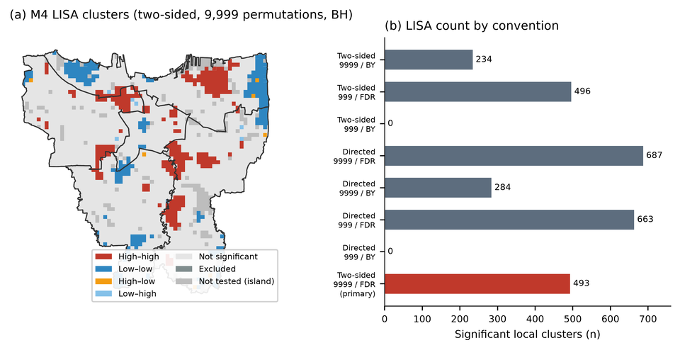
Local indicators of spatial association (LISA) use conditional randomisation with the same weights and seed. The adopted reporting convention is two-sided testing with 9,999 permutations and Benjamini–Hochberg (BH) correction at across all non-island cells in the M4 map. A two-sided test is used because both positive spatial clusters and spatial outliers are relevant to reading the map; the study is exploratory and the convention was adopted during analysis, not preregistered. The 9,999 permutations give a minimum attainable -value of 0.0001. We report directed testing, 999 permutations and Benjamini–Yekutieli (BY) correction as sensitivity analyses. BH controls the false discovery rate under independence or positive dependence; BY is more conservative under arbitrary dependence. The testing family is each preselected map separately, not a family across all interactive selections. A local cluster label is not evidence that the index is valid, that the cluster is a social process, or that an intervention would be effective. Table 10 reports the convention range.
4.8Scenario envelope and reproducibility
The scenario registry contains 52 scenarios in families covering weights (9 scenarios), park thresholds (4), normalisation (3), QA exclusions (3), route policy (5), thermal support (2), land cover (1), population specification (2), joint factorial combinations (16) and other variants. Two families (entrance/barrier and thermal sampling) could not be evaluated because the required evidence was unavailable; the temporal family is conditional on historical data that could not be reconstructed. We report the minimum and maximum Jaccard within each family at the 10% budget. The joint factorial is a 16-scenario subset crossing construct, cap, normalisation and aggregation choices; route-policy variants are a separate family. We therefore do not claim all-family robustness. The purpose of the envelope is to show which conclusions survive plausible alternatives and which do not.
The analysis is reproducible from the processed outputs and pipeline at commit 3b8ed05be92c35bbb2b3a617688540ee856b11c8 (implementation SHA-256 6b2eae9dc37b14d92bd6accafda602da1e42af643ba8a72b6431d60e985b233e). The processed dataset contains 2,765 master cells, 2,536 common eligible cells and 254 top-decile rows per model. Two independent builds reproduced 63 tables with a maximum numerical difference of 0.0. A clean-checkout test suite passed (236 tests plus 7 subtests), and the standard and remediation output manifests were portable (69/69 and 80/80 relative paths). These checks concern software reproducibility, not the scientific validity of the index. Exact commands, input hashes and output hashes are reported in the reproducibility note and in the Data and Code Availability section.
5Results
5.1Environmental, demographic and accessibility distributions
The common sample has a mean LST of 41.49 C (SD 2.29; range 31.28–47.92), a mean NDVI of 0.315 (SD 0.106; range –0.795), and a modelled population of 10.52 million people (mean 4,148 per cell; median 4,288). Children and older adults account for 3.11 million people, or 29.5% of the modelled population, with a between-cell share that is remarkably narrow (mean 0.2955, SD 0.0073, 5th–95th percentile 0.2894–0.3016). This narrowness is the first indication that an age-count term will behave almost like a population term.
Candidate-park distance is available for all 2,536 common cells: 537 are within 500 m, 1,390 are within 1,000 m (including the 537), and 1,146 are beyond 1,000 m. The mean distance is 1,141.6 m (median 909.0 m; 95th percentile 2,922.2 m; maximum 5,756.0 m). The distribution is right-skewed, and the 1,000 m cap used by M4 compresses 45.2% of the common sample into the maximum-deficit category. Figure 1 maps LST and NDVI; Figure 2 maps population and candidate-park distance. The maps show the expected broad pattern of hotter, less vegetated central and northern areas, but they also show substantial cell-to-cell heterogeneity that a city-level summary would obscure.
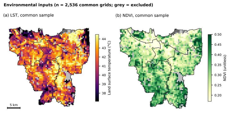
merged_grid.csv and priority_models.csv from the processed analysis tables; figure generated for this manuscript from those tables.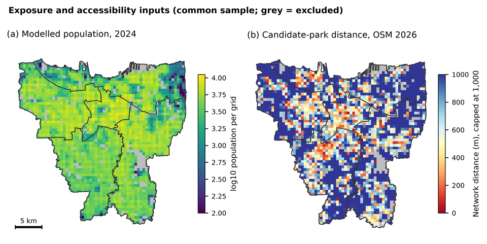
merged_grid.csv and priority_models.csv.5.2Baseline priority patterns under M1–M4
Each model assigns 254 cells to its top decile. The score distributions shift upward and become narrower as components are added: M1 has mean 0.598 (SD 0.268), M2 0.585 (0.247), M3 0.631 (0.227) and M4 0.669 (0.173). The compression is partly a consequence of adding components with different distributions and partly a consequence of percentile clipping. M4 has only two cells tied at the maximum, compared with 127 for M1, so the top of the M4 ranking is less saturated.
The geography of the top decile changes substantially across models. Under M1, the top decile is concentrated in East Jakarta (88 cells, 34.6% of the top set) and North Jakarta (77, 30.3%), with 48 in South Jakarta, 39 in West Jakarta and only 2 in Central Jakarta. Under M4, East Jakarta still contributes 87 cells (34.3%), but West Jakarta rises to 63 (24.8%), Central Jakarta to 17 (6.7%), while South Jakarta falls to 32 (12.6%) and North Jakarta to 55 (21.7%). The M4 top decile contains 1.54 million people, or 14.6% of the common-sample population, and 63.4 km of land. M1’s top decile contains 1.37 million people and 62.6 km. The difference in population share is modest, but the geographic redistribution is not.
Figure 3 maps the M1 and M4 top deciles. The two maps share a broad belt of high priority in the north-east and along parts of the eastern and southern fringe, but they disagree on many cells in the west and centre. This is the visual counterpart of the low Jaccard overlap reported below. The maps are screening maps: a red cell is a candidate for further investigation, not a validated intervention site.
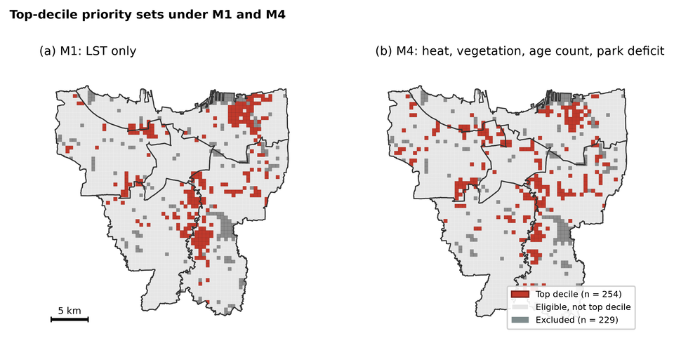
5.3Ranking displacement and top-priority change
Model agreement is high in rank correlation but modest in top-set overlap. Spearman’s is 0.936 between M1 and M2, 0.905 between M1 and M3, and 0.847 between M1 and M4. Kendall’s follows the same order (0.782, 0.736 and 0.658). The M3–M4 correlation is 0.898 (), which might suggest substantial agreement; the top-decile Jaccard is only 0.411. The difference between these statements is the difference between a global rank correlation and a boundary-sensitive set comparison. A correlation of 0.9 can coexist with a large change in which cells cross the top-decile threshold.
The M1-to-M4 mean absolute rank shift is 307 positions (median 239; 90th percentile 696.5; maximum 1,714) on a 2,536-cell ranking. Almost half of the cells (48.3%) move by more than 10% of the ranking, and only 0.3% retain the same rank. The M3-to-M4 shift is smaller but still large: mean 266.7, median 248, 90th percentile 487, maximum 1,065. M1-to-M2 shifts are smaller (mean 199.6, median 156), and M2-to-M3 shifts are the smallest (mean 129.0, median 88). The ordering is intuitive: adding vegetation to LST changes the ranking less than adding population, and adding population changes it less than adding park distance and age.
Top-set overlap depends strongly on the budget. At the 5% budget, M1–M4 Jaccard is 0.316, with 61 of 127 cells shared (48.0% retention); at 10% the Jaccard is 0.384, with 141 of 254 cells shared (55.5% retention); at 20% the Jaccard is 0.488, with 333 of 508 cells shared (65.6% retention). M3–M4 Jaccard is 0.419, 0.411 and 0.532 at the same budgets. M2–M3 is the most stable pair (0.649, 0.688 and 0.758). The top-decile comparison is therefore not a generic statement that "the models disagree"; it is a statement that the disagreement is concentrated near the priority boundary, where small score changes can move a cell in or out of the set. Jaccard and retention answer different questions: Jaccard divides the shared cells by the union, whereas retention divides them by the size of one set. Figure 4 shows the displacement and its distribution.
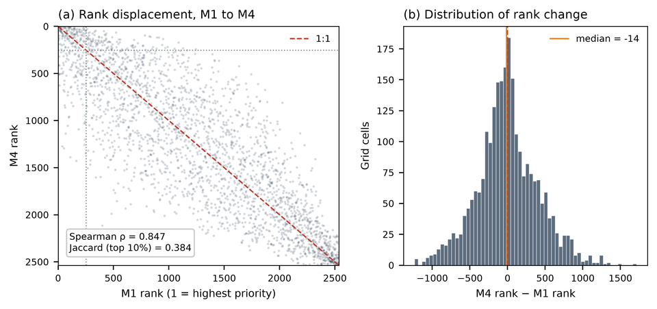
priority_models.csv.| Pair | Spearman | Kendall | Mean rank | |||
|---|---|---|---|---|---|---|
| M1–M2 | 0.936 | 0.782 | 0.477 | 0.568 | 0.693 | 199.6 |
| M1–M3 | 0.905 | 0.736 | 0.330 | 0.481 | 0.590 | 235.5 |
| M1–M4 | 0.847 | 0.658 | 0.316 | 0.384 | 0.488 | 307.4 |
| M2–M3 | 0.964 | 0.856 | 0.649 | 0.688 | 0.758 | 129.0 |
| M2–M4 | 0.882 | 0.701 | 0.403 | 0.392 | 0.523 | 283.5 |
| M3–M4 | 0.898 | 0.736 | 0.419 | 0.411 | 0.532 | 266.7 |
All correlations are computed on the same 2,536 cells. At the 10% budget, the shared-cell counts and retention relative to either 254-cell set are: M1–M2 184 (72.4%), M1–M3 165 (65.0%), M1–M4 141 (55.5%), M2–M3 207 (81.5%), M2–M4 143 (56.3%), M3–M4 148 (58.3%). Jaccard divides the shared cells by the union, so it is lower than retention; for M1–M4, . High rank correlation can coexist with low Jaccard because the top decile is a boundary-sensitive set. Jaccard values are sensitive to the budget and should not be generalised beyond the stated threshold.
5.4Attribution of M3-to-M4 change
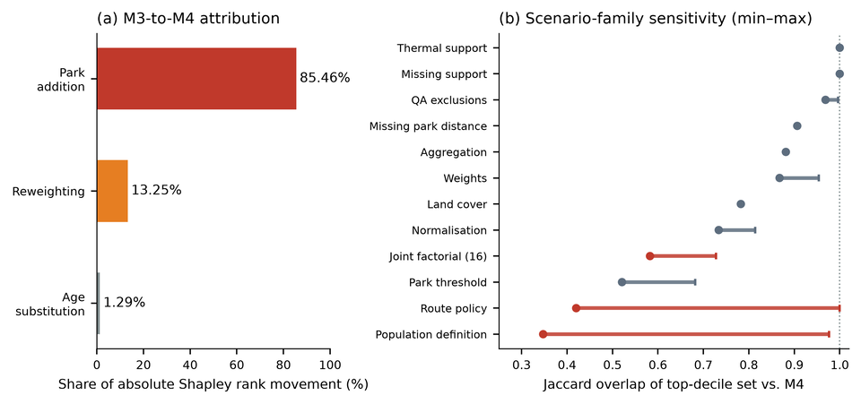
The exact Shapley decomposition attributes 85.46% of the absolute M3-to-M4 rank movement to park addition, 13.25% to reweighting and 1.29% to the age substitution. The shares are normalized absolute contributions; they describe the model change, not the real-world importance of parks, age or vegetation. The park share is large because the park term is new, enters at a 0.25 weight, and has a wide 0–1 range that is not compressed by percentile clipping. The age share is small because the age count is nearly proportional to total population and the weight change is modest.
The matched-weight incremental comparisons are relative to M3 and are reported in Table 7. Adding the park term while holding the other weights fixed yields a top-decile Jaccard of 0.490 against M3 (167 of 254 cells shared). Reweighting alone yields 0.961 (249 shared), and the age swap alone yields 0.984 (252 shared). Adding park plus reweighting yields 0.415; age plus park yields 0.499; all three changes yield 0.411. These values answer how much each change moves the M3 top set; they are not similarities to M4.
The same scenarios compared with M4 are reported in Table 8. Park addition alone is the closest single change to M4 (Jaccard 0.861; 235 of 254 cells shared), while reweighting alone (0.423; 151 shared) and the age swap alone (0.419; 150 shared) are much further away. Park plus reweighting reaches 0.977, and age plus park reaches 0.847. Read together, the two tables show that the park term is the dominant source of set change, but the numbers are not interchangeable: Jaccard divides shared cells by the union of the two sets, whereas retention divides them by one set’s size.
The construct ablations relative to M4 are also in Table 8. A park-only index has a top-decile Jaccard of 0.028 with M4 (14 of 254 cells shared), showing that M4 is not merely a park map; a no-park variant has Jaccard 0.423, and a heat-only variant 0.384. An equal-weight variant has Jaccard 0.868, and a proportional M3-plus-park variant 0.924. These benchmarks are internal comparisons on the same sample, not external validation. Figure 5 shows the Shapley shares and the scenario-family envelope.
rank_change_attribution.csv and robustness_family_summary.csv.| Scenario | Jaccard vs M3 | Shared / 254 | Interpretation |
|---|---|---|---|
| M3 (reference) | 1.000 | 254 | M3 top decile |
| Reweighting only | 0.961 | 249 | Changes weights but keeps M3 components |
| Age swap only | 0.984 | 252 | Replaces total population with age count |
| Park addition only | 0.490 | 167 | Adds park term at matched weights |
| Age + reweighting | 0.954 | 248 | Joint change without park |
| Park + reweighting | 0.415 | 149 | Park dominates the joint change |
| Age + park | 0.499 | 169 | Park plus age substitution |
| M4 (all three changes) | 0.411 | 148 | Full M3-to-M4 construct change |
These are incremental comparisons against M3. They answer: how much does each change move the M3 top set? The corresponding M4-referenced comparisons are in Table 8; the same numerical Jaccard cannot be interpreted as both an M3 and an M4 overlap. The exact three-factor Shapley shares are 85.46% park, 13.25% reweighting and 1.29% age; these are descriptive shares of absolute rank movement, not causal effects.
| Scenario | Jaccard vs M4 | Shared / 254 | Interpretation |
|---|---|---|---|
| M4 (reference) | 1.000 | 254 | Full screening index |
| M3 | 0.411 | 148 | Removes age count and park term; reweights |
| Reweighting only | 0.423 | 151 | Changes weights but keeps M3 components |
| Age swap only | 0.419 | 150 | Replaces total population with age count |
| Park addition only | 0.861 | 235 | Adds park term at matched weights |
| Age + reweighting | 0.423 | 151 | Joint change without park |
| Park + reweighting | 0.977 | 251 | Park dominates the joint change |
| Age + park | 0.847 | 233 | Park plus age substitution |
| No park | 0.423 | 151 | Removes park term from M4 |
| Park only | 0.028 | 14 | Index based only on park deficit |
| Heat only | 0.384 | 141 | M1 benchmark |
| Equal weight | 0.868 | 236 | Equal weights on four components |
| Total-count swap | 0.977 | 251 | Replaces age count with total population |
| Vulnerable share | 0.347 | 131 | Replaces count with age share |
| Child share | 0.451 | 158 | Child share instead of count |
| Elderly share | 0.392 | 143 | Elderly share instead of count |
| Proportional M3 + park | 0.924 | 244 | Reweights M3 components, adds park |
These are similarity comparisons against the M4 top decile. They answer: how close is each alternative specification to M4? They are not incremental changes from M3. The exact Shapley shares are in Table 7. “Shared” counts cells in both the scenario and M4 top sets.
5.5Accessibility-assumption sensitivity
Park-access assumptions change the top decile materially. The positive-tag-only destination scenario, which retains only 10 destinations, produces a top-decile Jaccard of 0.420 against the baseline when eligibility changes and 0.425 when anchors are fixed. This is a stress test, not a better estimate: the positive-tag set is sparse, and 2,482 cells are saturated at the 1,000 m cap. The conservative connector scenario, which removes 24,370 directed edges and increases missing routes to 407, produces a fixed-set Jaccard of 0.896. The baseline itself has 226 missing routes. The difference between 0.420 and 0.896 is the difference between a destination-coverage stress and a permission stress; both are plausible under different evidence assumptions, and neither is ground truth.
The missing-route bounds are also informative. Assigning the 1,000 m cap to missing routes (the worst-case deficit) and assigning the observed median distance (a neutral alternative) produce different top sets; the scenario family spans Jaccard 0.906 at the 10% budget. This is smaller than the destination stress but not negligible. The 13 route-missing cells that could enter the top 254 under a zero-deficit assumption are a further boundary uncertainty; they are not included in the common set and are mapped in the supplementary material. The 18 cells that are in the full-thermal M1 top 277 but lost from the common set are all route-missing (15 North, 2 East, 1 South). These cells are not evidence that the common set is representative; they are evidence that route missingness is spatially structured.
5.6Demographic-specification sensitivity
The demographic specification matters more for interpretation than for the primary ranking. Replacing the age count with total population at the same weight leaves the top decile almost unchanged (Jaccard 0.977; 251 of 254 retained). This is consistent with the near-collinearity of the two counts (Spearman ). The age count is therefore a population-weighted exposure term, not a distinct age-vulnerability signal. Replacing the count with a vulnerable share changes the set substantially (Jaccard 0.347; 131 retained). Child share yields 0.451 and elderly share 0.392. The share variants answer a different question: where vulnerable groups are a larger fraction of residents, not where many vulnerable people live. The primary M4 answers the latter question only.
The distinction is visible in the data. The vulnerable share is almost constant across the common sample (mean 0.2955, SD 0.0073), and its correlation with LST is essentially zero (Spearman ). The top-M4 cells have a vulnerable share of 0.2894–0.3016, a range of 1.2 percentage points. A model that claimed to identify age-vulnerable heat inequality on the basis of this term would be overstating what the data contain. The share scenario is useful precisely because it shows that a composition-oriented objective produces a different geography; it is not a correction that makes M4 better.
5.7The mechanical park-threshold effect
Under M4, the top-decile cutoff is 0.873739849. The maximum M4 score among the 537 common cells within 500 m of a candidate park is 0.869648776. The cutoff exceeds that maximum by 0.004091, so no near-park cell enters the top 254. The closest top-decile cell is 638.2 m from a candidate park; 174 of the 254 top cells are at the 1,000 m cap, and the remaining 80 are between 638 and 1,000 m. This is a property of the additive index and the observed input distribution, not an independently validated empirical discovery that the most heat-vulnerable places lack parks.
A concrete case illustrates the arithmetic. Cell JKT_R056_C048 in North Jakarta has an LST of 45.58 C, a modelled population of 6,971 and a candidate-park distance of 487.96 m. Its M4 score is 0.869649 and its rank is 274, just outside the top 254. Of the 254 top cells, 236 are cooler than this cell. The model is not "wrong" in the sense of an arithmetic error; it is doing what the additive formula specifies. But the result is a screening priority that penalizes a hot, populous, near-park cell because the park term contributes only 0.122 while the other components do not compensate enough to cross the cutoff. Presenting this as evidence that parks do not matter, or that near-park residents are not heat-vulnerable, would invert the meaning of the model.
5.8Missing-data exclusions and representativeness
The 229 excluded cells account for 8.28% of the master grid and 4.22% of the modelled population (463,697 people). They are not a random subset. Included cells have a mean LST of 41.486 C, mean NDVI 0.315, mean coverage 0.940 and mean snapping distance 49.98 m. Excluded cells have a mean LST of 40.283 C, mean NDVI 0.365, mean coverage 0.821 and mean snapping distance 98.81 m. The excluded cells are therefore cooler, greener, more peripheral and less well connected (Table 9). Their city distribution is East Jakarta 96, North Jakarta 77, South Jakarta 28, West Jakarta 22 and Central Jakarta 6. Most are route-missing (226 of 229), with two population-only exclusions and one low-LST exclusion.
This profile has two consequences. First, the common-set estimate is conditional on the included cells; it is not a Jakarta-wide estimate. Second, the excluded cells are not uniformly low-priority: 18 cells that are in the full-thermal M1 top 277 are lost from the common set, and 13 route-missing cells could enter the top 254 under a zero-deficit assumption. The common-set map should therefore be read alongside the exclusion map in the supplementary material. A priority map that omits the excluded cells without showing them invites the reader to mistake the study area for the city.
| Group | Cells | Population | Mean LST (C) | Mean NDVI | Mean coverage | Mean snap (m) |
|---|---|---|---|---|---|---|
| Included (common) | 2,536 | 10,519,841 | 41.486 | 0.315 | 0.940 | 49.98 |
| Excluded | 229 | 463,697 | 40.283 | 0.365 | 0.821 | 98.81 |
Excluded cells account for 8.28% of the master grid and 4.22% of the modelled population. The exclusion is spatially structured: East Jakarta 96, North Jakarta 77, South Jakarta 28, West Jakarta 22 and Central Jakarta 6. These cells are not a random sample and the common-set estimate is not Jakarta-wide.
5.9Global and local spatial clustering
Global Moran’s is positive and highly significant for all four models under the permutation convention: M1 0.6711, M2 0.6540, M3 0.6644 and M4 0.5930, with in every case. The expected value under randomization is . The M4 value is lower than M1–M3, consistent with the addition of a park term that is less spatially smooth than LST. The -value of 0.001 is the minimum attainable at 999 permutations; it should be read as , not as .
Local cluster labels are materially convention-dependent. Under the adopted two-sided/9,999/BH convention, the M4 map has 252 high–high, 227 low–low, 7 high–low and 7 low–high cells, with 493 significant cells and 2,042 non-significant cells. The historical directed/999/BH configuration yields 663 significant cells (319 high–high, 323 low–low, 11 high–low and 10 low–high; 1,872 non-significant). Two-sided testing at 999 permutations yields 496 significant cells; directed testing at 9,999 permutations yields 687. BY correction at 999 permutations yields zero significant cells, because the minimum attainable -value (0.001) exceeds the BY threshold (); at 9,999 permutations it yields 284 directed and 234 two-sided significant cells. The zero is a resolution artifact, not evidence that no local clustering exists.
Figure 6 maps the M4 clusters under the adopted convention and shows the count range across alternatives. The map is useful for exploring spatial structure, but it is not a validated cluster map. A different tail, permutation count or correction changes which cells are labelled. We therefore report the full range and avoid statements such as "significant everywhere" or "no significant clusters" without naming the convention.
lisa_tail_permutation_grid.csv, lisa_m4_primary.csv and lisa_tail_permutation_sensitivity.csv.| Tail | Permutations | Correction | Significant cells | Changed vs primary |
|---|---|---|---|---|
| Two-sided | 9,999 | BH | 493 | 0 |
| Two-sided | 999 | BH | 496 | 65 |
| Directed | 999 | BH | 663 | 170 |
| Directed | 9,999 | BH | 687 | 194 |
| Two-sided | 9,999 | BY | 234 | 259 |
| Directed | 9,999 | BY | 284 | 209 |
| Directed | 999 | BY | 0 | 493 |
BH: Benjamini–Hochberg at ; BY: Benjamini–Yekutieli at . At 999 permutations the minimum attainable -value is 0.001. The BY threshold at 999 permutations is approximately , so the zero count is a resolution artifact, not evidence of no clustering. No claim is made; normal-theory -value underflow is not used as evidence. The directed/999/BH column is retained as the historical analytical configuration.
5.10Scenario envelope and stability
The scenario envelope shows partial stability, not uniform robustness. At the 10% budget, the aggregation family has Jaccard 0.881; QA exclusions 0.969–0.996; missing support 1.000; thermal support 1.000; land cover 0.782; normalisation 0.734–0.814; park threshold 0.521–0.682; weights 0.868–0.954; population definition 0.347–0.977; route policy 0.420–1.000; and the 16-scenario joint factorial 0.583–0.728. The joint factorial never reaches 0.8, and the route and population families contain the lowest values. A claim that "the priorities are robust" is therefore not supported. A more accurate statement is that a subset of cells is stable across several families, while the boundary of the top decile is contingent on construct, weight, demographic and access choices.
The stability map in the supplementary material shows this subset. It should not be read as a validated core: stability across the scenarios we happened to run is not stability across all plausible models. The scenario registry itself is a choice, and two families (entrance/barrier and thermal sampling) could not be evaluated because the required evidence was unavailable. The envelope is an honest description of the sensitivity we could test, not a complete uncertainty budget.
| Family | Scenarios | Minimum | Maximum |
|---|---|---|---|
| Aggregation (hybrid vs fractional) | 1 | 0.881 | 0.881 |
| Park threshold (500 m, 1,000 m, caps) | 4 | 0.521 | 0.682 |
| Weights (including equal weight) | 9 | 0.868 | 0.954 |
| QA exclusions (snap, coverage) | 3 | 0.969 | 0.996 |
| Missing park distance (median, cap) | 2 | 0.906 | 0.906 |
| Joint factorial (construct, cap, normalisation, aggregation) | 16 | 0.583 | 0.728 |
| Missing support | 1 | 1.000 | 1.000 |
| Normalisation (min–max, rank) | 3 | 0.734 | 0.814 |
| Population definition (count vs share) | 2 | 0.347 | 0.977 |
| Route policy (baseline, conservative, positive tags) | 5 | 0.420 | 1.000 |
| Thermal support (0.50, 0.25, strict) | 2 | 1.000 | 1.000 |
| Land cover (tree probability) | 1 | 0.782 | 0.782 |
Jaccard values are computed against the baseline M4 top decile with the scenario’s eligible set (eligibility-changing comparison). The joint factorial does not include route-policy variants, so the table does not support an all-family robustness claim. Two further families (entrance/barrier and thermal sampling) could not be evaluated because the required evidence was unavailable, and they are not reported as estimates.
5.11Summary of the evidence
Three results are robust in the sense that they follow from exact arithmetic and do not depend on interpretive choices. First, M1 and M4 produce materially different top-decile sets (Jaccard 0.384) despite a high rank correlation (0.847). Second, the age count is nearly collinear with total population (), and a total-count swap leaves the top decile almost unchanged (0.977), while a share swap changes it substantially (0.347). Third, under the observed M4 inputs, no cell within 500 m of a candidate park enters the top 254; the cutoff and the maximum near-park score differ by 0.0041.
Three further results are conditional. First, the attribution shares (85.5% park, 13.2% reweighting, 1.3% age) describe this M3-to-M4 configuration and should not be generalised to other weights or caps. Second, the access stress tests show that destination and permission assumptions can change the top set materially, but the positive-tag scenario is not ground truth. Third, the LISA labels are convention-dependent, and the range (0 to 687 significant cells) is too wide to support a single cluster narrative. These conditional results are still useful: they tell the analyst where the index is fragile and what evidence would be needed to resolve the fragility.
6Discussion
6.1Adding indicators changes the question, not just the map
The four models are often described as progressively "better" because they include more information. That framing is misleading. M1 answers a narrow question: where is the surface hottest? M2 asks where heat coincides with low vegetation. M3 asks where heat and vegetation coincide with many residents. M4 asks where heat, vegetation, a count of children and older adults, and a modelled park deficit combine into a high score. These are different questions, and none is a gold standard for the others. A cell that ranks first under M1 may rank 274th under M4 without either model making an arithmetic error. The appropriate question is not "which model is right?" but "which question is the decision supposed to answer, and how transparent is the value judgement embedded in the composite?"
This is especially important for policy communication. A heat-only map can be read as a physical hazard map. A composite map is read by many audiences as a vulnerability or priority map, even when its authors intend it as a screening device. The label matters. We therefore describe M4 as an exploratory heat–population–park-deficit screening index, not as a heat inequality or age-vulnerability index. The distinction is not semantic: it determines which claims are licensed by the output.
6.2Why the park term dominates
The park term dominates the M3-to-M4 rank movement for three structural reasons. First, it is new: the other components are present in M3 in some form, so the park term introduces a dimension that was previously absent. Second, it enters at a 0.25 weight, which is large relative to the 0.30/0.20 weights on LST and vegetation. Third, it is defined on a fixed 0–1 scale with a hard cap, whereas the other components are percentile-normalised and compressed near their central range. A cell at the cap receives the full 0.25 contribution; a cell at 500 m receives 0.125. The additive form makes these contributions tradeable against heat and population. The result is a ranking in which distance to a candidate park can outweigh a large LST difference.
None of this demonstrates that parks are unimportant. It demonstrates that the index is sensitive to the park term’s scale and weight. A different cap, a nonlinear distance decay, a binary threshold or a separate park-access model would produce a different ranking. The park term is a legitimate planning construct, but its dominance is a design property that should be disclosed, not a finding about the world. The near-park hot cell example is the clearest illustration: the model ranks a 45.6 C, 6,971-person cell outside the top 254 because its park deficit is small. A policymaker who reads the top decile as "the most heat-vulnerable places" would draw the wrong conclusion. A policymaker who reads it as "places where a particular additive screening rule scores high" would not.
6.3What the age term does and does not contribute
The age count contributes little beyond total population in this dataset. The two counts have a Spearman correlation of 0.9995, and replacing one with the other changes only 3 of 254 top cells. This is not because age is unimportant; it is because the age count is a population-scaled measure in a setting where the vulnerable share is nearly constant. A count answers "where are many vulnerable people?" and will therefore track population. A share answers "where are vulnerable people a larger fraction of residents?" and produces a different geography. The share variants have Jaccard 0.347–0.451 with M4, showing that the choice of estimand matters more than the choice of age group.
The policy implication is to separate the questions. If the goal is to find places with many older adults during a heat event, a count is defensible, but it should be labelled as population-weighted exposure rather than age vulnerability. If the goal is to test whether age composition is associated with heat, a share or a regression with population controls is needed. Mixing a count and a share in one composite, or interpreting a count as a composition, obscures the distinction. Our results support the first interpretation for M4 and reject the second.
6.4Why park-access evidence is uncertain
The park layer is a candidate inventory, not a verified public-access inventory. No destination has verified public access or a verified entrance; 980 of 1,015 are tagged unknown, and all 1,015 remain unresolved. OSM completeness and tagging quality vary, and a missing tag is not evidence of a closed park (52–54). The walking graph is also a model: origins and destinations are snapped to nearest nodes, park polygons are represented by representative points, and 167 origin connectors plus 78 park connectors conflict with explicit node restrictions. The conservative scenario removes 24,370 directed edges and increases missing routes to 407. The positive-tag-only scenario retains 10 destinations and saturates 2,482 cells at the cap. Neither scenario is a validated access measure.
This uncertainty is not a reason to discard the park term. It is a reason to report it as a proxy and to show the range. The baseline and conservative scenarios agree on a large share of the top decile (Jaccard 0.896), which is reassuring for the permission dimension. The destination stress is much larger (Jaccard 0.420), which is a warning that the candidate inventory itself is a major source of uncertainty. A field audit of access and entrances for the highest-impact destinations would reduce this uncertainty more than a more complex routing algorithm on unverified tags.
6.5Sample selection and geographic generalisation
The common sample excludes 229 cells (8.3%) and 4.2% of the modelled population. The excluded cells are cooler, greener, more peripheral and less well connected. This is not a random loss: it is a spatially structured selection driven by route missingness and source support. The common-set estimate is therefore conditional on the included cells, and the excluded cells should be shown on every priority map. The 18 full-thermal M1 top cells lost from the common set and the 13 route-missing cells that could enter the top 254 are not footnotes; they are part of the uncertainty of the map.
The appropriate language is "the five mainland cities under the common-set configuration", not "Jakarta". A Jakarta-wide claim would require either complete route coverage or an explicit imputation model for missing routes, and neither is available. The current analysis supports a conditional screening statement. It does not support a citywide prevalence estimate, a comparison of city-level rates, or a claim that the excluded periphery is unimportant. The periphery is cooler and greener on average, but it also contains hot cells and people, and the average masks that heterogeneity.
6.6Spatial inference and policy interpretation
The LISA results illustrate why spatial inference needs conventions. Under the adopted two-sided/9,999/BH convention the same M4 map yields 493 significant local clusters; the historical directed/999/BH configuration yields 663, the two-sided/999/BH configuration 496, directed/9,999/BH 687, and BY/999 zero. The zero is not a substantive finding; it is a consequence of the minimum attainable permutation -value and the BY threshold. A paper that reported only the largest number would overstate certainty; a paper that reported only the zero would understate it. The useful report is the range, with the adopted convention named and the alternatives disclosed.
Local clusters are also not causal processes. A high–high cluster of M4 scores can arise from the index’s own spatial structure, from the distribution of population, or from the park term. It does not identify a social mechanism, a health effect or a policy lever. The cluster map is an exploratory tool for generating hypotheses and for designing field work. It is not a substitute for an outcome model.
6.7Comparison with prior work
Our results overlap with prior work in several ways. The LST–NDVI relationship and the surface urban heat island literature justify the M1/M2 layers (1, 2, 27, 29). Heat vulnerability indices justify the demographic layers (7, 8). Network-access studies justify the park layer (22, 40, 44). Composite-indicator research justifies the sensitivity design (11, 12, 31). Jakarta studies establish the local relevance (3–5, 13). The contribution is not the combination of these ingredients. It is the quantitative attribution of how the combination changes priorities, the demonstration that an age count is nearly redundant with population, and the disclosure that an additive park term can mechanically determine the top decile.
The closest Jakarta comparator is Perdinan et al. (19). They integrate 30 m LST, vegetation deficit, built-up intensity and population density through an ordinary least-squares model, construct a weighted priority index, and evaluate four weighting scenarios and threshold relaxation. Their priority tiers remain structurally consistent, and high-LST clusters persist in dense built-up corridors. Their question is which vegetation-based adaptation tiers are robust to specification, whereas ours is how a sequence of screening constructs changes cell-level rankings and which component drives that change. The two findings are compatible: administrative priority tiers can remain similar while top-decile membership shifts substantially at the cell level. We do not present M4 as a better adaptation index than their regression-informed framework; we examine what the construction of a screening index does to its spatial priorities.
A second comparator treats disagreement itself as decision support. Fitria et al. (25) compare equal-weight and principal-component heat-vulnerability indices across 158 Taiwanese districts using 17 indicators, introduce a Spatial Disagreement Index, and find only moderate rank agreement (Spearman ) with disagreement concentrated in urban–rural fringe districts. Their leave-one-out analysis further shows that the two aggregation methods retain different shares of top-priority districts. This is a direct precedent for interpreting ranking differences as information rather than as noise. Our exact Shapley decomposition is complementary: it attributes a sequential M3-to-M4 transition rather than a contrast between two aggregation methods. We do not claim to be the first study to decompose or diagnose disagreement among heat-priority rankings.
Ramadhanis et al. (20) and Dong et al. (21) place demographic and accessibility evidence in a broader context. Ramadhanis et al. combine under-five population density with OSM green-space network distance in Jakarta and identify child-specific vulnerability concentrations, particularly in North, West and East Jakarta. Dong et al. use an improved two-step floating catchment area and bivariate local Moran’s I to compare cooling accessibility and heat-risk exposure in Zhengzhou. Both studies make accessibility or age-specific vulnerability the estimand. In our analysis, age and park distance are components of a screening index; the objects of inquiry are the redundancy of an age count with total population and the sensitivity of the ranking to modelled candidate-park destinations and routing. Our results therefore describe the behaviour of a screening construct, not verified public access or individual heat-health vulnerability.
Elmarakby and Elkadi (23) show how a district Heat Risk Index can prioritise UHI mitigation, and Ulfiasari and Yola (18) document a decade of UHI expansion in metropolitan Jakarta. These studies establish the planning relevance of composite risk mapping and the local physical signal. They do not ask how a sequential change in a screening index redistributes cell-level priorities. Compared with Sidiqui et al. (64), we use a finer grid, a network-based candidate-park measure and an explicit attribution decomposition, but we do not claim a better vulnerability map. Compared with Kim and Kwak (22), we do not implement a cooling-weighted G2SFCA or a demand-allocation model; our park term is a simpler distance deficit. Compared with Fung et al. (65), we do not evaluate heat-mitigation interventions; we evaluate how a screening index responds to specification choices. These differences define a narrower but defensible contribution.
6.8What a policymaker may legitimately infer
A policymaker may legitimately use the maps to generate a shortlist of cells for field inspection, to compare the spatial implications of different screening questions, and to see where the ranking is sensitive to assumptions. The maps can support a conversation about whether a park-access term should be included, how much weight it should receive, and what evidence would be needed to verify the candidate destinations. They cannot support a claim that a particular cell is the best place to invest, that a park would cool it by a specified amount, or that the top decile corresponds to excess mortality or morbidity. Those claims require outcome data, cooling-effectiveness estimates, cost data and a causal design that this study does not provide.
The most defensible policy use is procedural: require a sensitivity report alongside any composite priority map, show excluded and unknown cells, state the access construct, and separate screening from evaluation. The analysis documentation records the corresponding tables and sensitivity scenarios, but it does not replace scientific judgement.
6.9What remains unknowable from the present data
Several questions cannot be answered with the current evidence. We do not know the original 2024 acquisition dates, the seasonal representativeness of the thermal composite, or whether the 2026 park and network snapshot resembles the 2024 network. We do not know which candidate parks are publicly accessible, when they are open, whether they have entrances on the modelled network, or whether they provide cooling refuge. We do not know how many people use them, how far they actually walk, or how heat affects their health. We do not know whether the excluded cells would change the top decile if routes were resolved. These are not minor caveats; they define the boundary between a screening exercise and an impact evaluation.
7Limitations
The limitations of this study are specific and consequential.
- Thermal acquisition provenance. The original Earth Engine scene, task and AOI records are unavailable. The 2024 label is a declared recipe period, not a verified acquisition history. Scene counts, dates and seasonal sampling cannot be reconstructed from the delivered median raster. No annual, seasonal or trend claim is supported.
- LST is not air temperature or personal exposure. LST measures the radiant surface temperature of the skin of the city. It is not the air temperature a person experiences, and it does not incorporate humidity, wind, shade, clothing, activity or access to cooling. The relationship between LST and heat stress is context-dependent (6).
- Temporal composite representativeness. The median composite is built from unequal clear-observation counts across pixels (grid mean 5.96–27.4 observations per pixel in the delivered data). The median is not an annual mean, and the monthly/seasonal balance is unknown.
- Mixed reference periods. LST and demographic inputs refer to a declared 2024 period; the OSM park and pedestrian network is a 19 November 2026 snapshot. The analysis is a mixed-period candidate proxy, not a contemporaneous 2024 reconstruction.
- OSM park inventory coverage. The inventory contains 1,015 candidate polygons, but OSM completeness and tagging vary. Some public parks may be missing; some mapped polygons may not be parks. The candidate set is not a census.
- Unverified public access. No candidate has verified public access or a verified entrance. The 980 unknown, 28 conditional and 7 positive-tag classifications are evidence states, not access determinations. A positive tag is an unverified assertion.
- Unverified park entrances and connectors. Park polygons are represented by representative points, and origins and destinations are connected to the graph at nearest nodes. These connectors are not field-verified. The conservative scenario removes 24,370 directed edges and leaves 407 missing routes.
- Walking-network approximations. The graph is a pedestrian network derived from OSM. It does not encode opening hours, temporary closures, stairs, crossings, security gates, flooding or construction. Shortest-path distance is not the same as walkability or perceived access.
- Missing park distances. The baseline has 226 route-missing cells (8.2%). They are excluded, not assigned a distance. The conservative scenario has 407. The 13 route-missing cells that could enter the top 254 are a lower bound on the effect of missingness.
- Demographic raster support. Six cells remain unsupported in total population and both age groups, including two substantively large North Jakarta cells. They are retained as nulls, not zeros. The 13 recovered cells depend on buffered age surfaces and a hybrid aggregation rule.
- Population aggregation. The primary hybrid rule is not additive under repartitioning; the fractional alternative changes 16 top-M4 cells and has Jaccard 0.881 with the baseline. The hybrid allocation is retained for continuity; area-fractional allocation is the conceptually preferable alternative for additive population accounting.
- Partial coastal grids. 383 cells are partial polygons; 65 have less than 10% coverage. Small-area population and density estimates are uncertain, and the lattice clipping affects the spatial graph.
- Weighting and normalisation. The weights are a modelling choice, not estimates derived from Jakarta-specific evidence. Percentile clipping saturates scores and creates ties. The park cap is likewise a modelling choice. Different weights, caps or normalisation rules produce different rankings, as the scenario envelope shows.
- Sample selection. The common sample excludes 229 cells (8.3%) and 4.2% of the modelled population. Excluded cells are cooler, greener, more peripheral and less connected. The common-set estimate is conditional, not Jakarta-wide.
- Spatial inference conventions. LISA labels depend on tail, permutation count and multiple-testing correction. The adopted two-sided/9,999/BH convention yields 493 significant M4 cells; the alternatives we examined range from 0 to 687. The 9,999-permutation resolution limit is 0.0001, and the 999-permutation sensitivity has a 0.001 limit; neither is evidence of .
- Limits of causal interpretation. The models are spatial associations. They do not identify causal effects of parks, vegetation, population or age on heat exposure or health. They do not estimate intervention effectiveness, cost-effectiveness or distributional welfare.
- Raw-data portability. The raw WorldPop, OpenStreetMap and GraphML inputs are not redistributed in this preprint package and are not tracked in the manuscript repository; exact raw-input hashes require the separate research bundle. The processed tables and code reproduce the reported results. A clean-checkout test suite and relative-path output manifests are documented in the reproducibility note. These engineering checks do not make the raw bundle public and do not establish acquisition-level satellite provenance.
8Conclusion
This paper examined how spatial priorities for urban heat screening in Jakarta change when LST and vegetation are supplemented with population, age count and modelled park access. The answer is: substantially, and in ways that are not captured by a single correlation or a single map. M1 and M4 share 141 of their 254 top-decile cells (55.5% retention), but the Jaccard overlap is only 0.384 because each set contributes 113 unique cells; the mean absolute rank shift is 307 positions. The M3-to-M4 change is dominated by the park term (85.5% of absolute rank movement), with reweighting (13.2%) and the age substitution (1.3%) playing smaller roles. The age count is nearly collinear with total population; a count-to-count swap leaves the top decile almost unchanged, while a count-to-share swap changes it substantially. Under the observed M4 inputs, no cell within 500 m of a candidate park enters the top 254, because the top-decile cutoff exceeds the maximum near-park score. That is a property of the additive index, not evidence that parks are unimportant.
The study’s contribution is therefore an attribution and uncertainty audit, not a new integrated framework and not a validated vulnerability map. It shows which conclusions are robust to the assumptions we could test, which are contingent, and which cannot be evaluated with the available evidence. The most important negative findings are that an age-count term does not measure age composition, that an additive park-deficit term can mechanically determine the top decile, and that local cluster labels are convention-sensitive. These findings are useful precisely because they constrain what a screening map can be used to say.
The next scientific steps are clear. Recover or formally restrict the thermal acquisition lineage. Field-verify public access and entrances for the highest-impact candidate parks. Resolve or explicitly model the 226–407 missing routes. Separate the heat-plus-population question from the age-composition and park-access questions, rather than forcing one composite to answer all three. Report the sensitivity of local inference to the LISA convention. Until those steps are completed, the present results should be read as a reproducible exploratory screening analysis, not as a validated risk model or a policy recommendation.
Author Contributions
All authors contributed to the preparation and critical revision of the manuscript. All authors reviewed and approved the final version and accept responsibility for its content.
Funding
This research received no external funding.
Conflicts of Interest
The authors declare no competing interests.
Data and Code Availability
Processed grid tables, model outputs, figure-generation scripts and the LaTeX source are held in the project’s research repository and are available from the corresponding author on reasonable request. The repository is not currently publicly archived, and no dataset DOI has been assigned. The raw WorldPop, OpenStreetMap and GraphML inputs are subject to their source licences and are not redistributed in this preprint package. WorldPop data are subject to CC BY 4.0 (63); OpenStreetMap data are subject to the Open Database License and attribution requirements (66). Original Landsat acquisition records were not available for independent verification, but the raster-to-grid aggregation can be reproduced from the retained exports. The study is therefore presented as an exploratory screening and sensitivity analysis conditional on these provenance limits, not as verified historical heat exposure or personal temperature exposure.
Technical reproducibility documentation records the analysis environment (Python 3.12.10; pandas 3.1.1; numpy 2.5.5; geopandas 1.2.0; libpysal 4.15.1; esda 2.10.0), software revisions, input and output hashes, clean-checkout test results, manifest paths and the two-build table replay. These records concern computational reproducibility and do not establish acquisition-level satellite provenance.
Acknowledgements
The manuscript uses the Manuscript Multi-Target LaTeX Template v1.0.0 by Rodolfo Aramayo (67) (DOI 10.5281/zenodo.22018962), distributed under GPL-3.0-or-later. The template’s class and bibliography style derive from Ricardo Henriques’s HenriquesLab bioRxiv template; upstream attribution is retained in the licence and provenance files. We thank the contributors to Landsat, WorldPop, OpenStreetMap, Python, GeoPandas, libpysal and esda.
Supplementary Material
The supplementary PDF contains: (S1) a data-quality and missingness register; (S2) scenario-family results at 5%, 10% and 20% budgets; (S3) city-level composition of the top deciles; (S4) alternative LISA summaries; (S5) the exclusion map and score distributions; (S6) all 49 executed scenario comparisons; (S7) the six demographic no-support cells; (S8) the master-to-common eligibility reconciliation; and (S9) figure and table provenance with the machine-readable supplementary files. The main text reports the results needed for the argument; the supplement documents the sensitivity detail and source support that would otherwise interrupt it.
Use of AI-Assisted Tools
AI-assisted tools were used for language editing, LaTeX production and consistency checking during the preparation of this manuscript. The authors reviewed and approved all scientific content and accept responsibility for the final article.
License
Copyright © 2026 The Authors. This work is licensed under a Creative Commons Attribution 4.0 International License (CC BY 4.0, https://creativecommons.org/licenses/by/4.0/). The licence applies to the author-created manuscript text, original figures and original supplementary narrative. Third-party datasets, software and the LaTeX template remain under their own licences and attribution requirements; the template source remains under GPL-3.0-or-later.
References
References
- T. R. Oke. The energetic basis of the urban heat island. Quarterly Journal of the Royal Meteorological Society, 108 (455): 1–24, 1982. doi: 10.1002/qj.49710845502.
- J. A. Voogt and T. R. Oke. Thermal remote sensing of urban climates. Remote Sensing of Environment, 86 (3): 370–384, 2003. doi: 10.1016/S0034-4257(03)00079-8.
- Siswanto Siswanto, Danang Eko Nuryanto, Muhammad Rezza Ferdiansyah, Agita Devi Prastiwi, and O. C. Dewi. Spatio-temporal characteristics of urban heat island of Jakarta metropolitan. Remote Sensing Applications: Society and Environment, 32: 101062, 2023. doi: 10.1016/j.rsase.2023.101062.
- C. D. Putra, A. Ramadhani, and E. Fatimah. Increasing urban heat island area in Jakarta and its relation to land use changes. IOP Conference Series: Earth and Environmental Science, 737 (1): 012002, 2021. doi: 10.1088/1755-1315/737/1/012002.
- Amalia Rakhmawati Rizki, Sri Setiawati Tumuyu, and Siti Badriyah Rushayati. The impact of urban green space on the urban heat island phenomenon: a study case in East Jakarta, Indonesia. Geoplanning: Journal of Geomatics and Planning, 11 (1): 31–42, 2024. doi: 10.14710/geoplanning.11.1.31-42.
- Nina Schwarz, Uwe Schlink, Ulrich Franck, and Katrin Großmann. Relationship of land surface and air temperatures and its implications for quantifying urban heat island indicators. Ecological Indicators, 18: 693–704, 2012. doi: 10.1016/j.ecolind.2012.01.001.
- Colleen E. Reid, Marie S. O’Neill, Carina J. Gronlund, Shannon J. Brines, Daniel G. Brown, Ana V. Diez-Roux, and Joel Schwartz. Mapping community determinants of heat vulnerability. Environmental Health Perspectives, 117 (11): 1730–1736, 2009. doi: 10.1289/ehp.0900683.
- Tanja Wolf and Glenn McGregor. The development of a heat wave vulnerability index for London, United Kingdom. Weather and Climate Extremes, 1: 59–68, 2013. doi: 10.1016/j.wace.2013.07.004.
- Sharon L. Harlan, Anthony J. Brazel, Lela Prashad, William L. Stefanov, and Larissa Larsen. Neighborhood microclimates and vulnerability to heat stress. Social Science & Medicine, 63 (11): 2847–2863, 2006. doi: 10.1016/j.socscimed.2006.07.030.
- Jacek Malczewski. Gis-based multicriteria decision analysis: a survey of the literature. International Journal of Geographical Information Science, 20 (7): 703–726, 2006. doi: 10.1080/13658810600661508.
- Michaela Saisana, Andrea Saltelli, and Stefano Tarantola. Uncertainty and sensitivity analysis techniques as tools for the quality assessment of composite indicators. Journal of the Royal Statistical Society: Series A (Statistics in Society), 168 (2): 307–323, 2005. doi: 10.1111/j.1467-985X.2005.00350.x.
- Salvatore Greco, Alessio Ishizaka, Menelaos Tasiou, and Gianpiero Torrisi. On the methodological framework of composite indices: a review of the issues of weighting, aggregation, and robustness. Social Indicators Research, 141 (1): 61–94, 2019. doi: 10.1007/s11205-017-1832-9.
- Alvin Christopher G. Varquez, Nisrina S. Darmanto, Yasushi Honda, Tomohiko Ihara, and Manabu Kanda. Future increase in elderly heat-related mortality of a rapidly growing asian megacity. Scientific Reports, 10: 9304, 2020. doi: 10.1038/s41598-020-66288-z.
- Safira Salsabila, Sulfikar Amir, and Anindrya Nastiti. Cooling as social practice: heat mitigation and the making of communal space in Jakarta’s informal settlements. Habitat International, 140: 102924, 2023. doi: 10.1016/j.habitatint.2023.102924.
- Jennifer R. Wolch, Jason Byrne, and Joshua P. Newell. Urban green space, public health, and environmental justice: the challenge of making cities “just green enough”. Landscape and Urban Planning, 125: 234–244, 2014. doi: 10.1016/j.landurbplan.2014.01.017.
- Alessandro Rigolon. A complex landscape of inequity in access to urban parks: a literature review. Landscape and Urban Planning, 153: 160–169, 2016. doi: 10.1016/j.landurbplan.2016.05.017.
- E. Dinand Ekkel and Sjerp de Vries. Nearby green space and human health: evaluating accessibility metrics. Landscape and Urban Planning, 157: 214–220, 2017. doi: 10.1016/j.landurbplan.2016.06.008.
- Sofi Ulfiasari and Lin Yola. Towards climate change adaptive spatial planning: Urban heat islands distribution in jakarta metropolitan area. In Elham Maghsoudi Nia, Iman Farshchi, Lin Yola, and Mokhtar Awang, editors, Sustainable Development Approaches: Selected Papers of AUA and ICSGS 2021, volume 243 of Lecture Notes in Civil Engineering, pages 111–118. Springer, Cham, 2022. doi: 10.1007/978-3-030-99979-7_13.
- Perdinan, Rahmad Fauzi, Rangga Agus Fauzi, Hadi Susilo Arifin, Delta Yova Dwi Infrawan, Yudi Setiawan, Prita Ayu Permatasari, Lasriama Siahaan, Aulia Fathiarahmah, and Mirza Shahreza. Spatial prioritization of vegetation-based climate adaptation pathways in tropical megacity jakarta, indonesia. Scientific Reports, 16 (1): 20857, 2026. doi: 10.1038/s41598-026-50579-y.
- Zainab Ramadhanis, Shofi Latifah Nuha Anfaresi, and Rani Fitri Febriyanti. Spatial assessment of children’s vulnerability to green space accessibility in jakarta, indonesia. Jurnal Pengembangan Kota, 14 (1): 72–83, 2026. doi: 10.14710/jpk.14.1.72-83.
- Xinyu Dong, Xiaoya Li, Yanmei Ye, Dan Su, Runjia Yang, and Angela Lausch. Measuring urban thermal environment from accessibility-based perspective: A case study in a populous city. Geography and Sustainability, 5 (3): 329–342, 2024. doi: 10.1016/j.geosus.2024.02.004.
- Wansu Kim and Yoonshin Kwak. A decision-support framework for equitable urban green space planning: cooling-weighted park accessibility for older adults. Land, 15 (6): 989, 2026. doi: 10.3390/land15060989.
- Esraa Elmarakby and Hisham Elkadi. Prioritising urban heat island mitigation interventions: Mapping a heat risk index. Science of the Total Environment, 948: 174927, 2024. doi: 10.1016/j.scitotenv.2024.174927.
- Saeideh Sobhaninia, Sara Meerow, Aubrey Dugger, Thomas Hopson, Cenlin He, et al. Where should the green go? a systematic literature review of methods for siting green infrastructure. Urban Forestry & Urban Greening, 107: 128790, 2025. doi: 10.1016/j.ufug.2025.128790.
- Laili Fitria, Da-Wei Tsai, Sheng-Jie You, and Ya-Fen Wang. Spatial disagreement as decision-support for district-level heat adaptation priorities: Evidence from taiwan’s six major cities. Sustainable Cities and Society, 148: 107630, 2026. doi: 10.1016/j.scs.2026.107630.
- Jakarta Heat Inequality Mapper Project. Jakarta heat inequality mapper: research data and analysis documentation. Project documentation, 2026. Project documentation; no public DOI assigned.
- Qihao Weng, Dengsheng Lu, and Jacquelyn Schubring. Estimation of land surface temperature–vegetation abundance relationship for urban heat island studies. Remote Sensing of Environment, 89 (4): 467–483, 2004. doi: 10.1016/j.rse.2003.11.005.
- Shushi Peng, Shilong Piao, Philippe Ciais, Pierre Friedlingstein, Liming Zhou, and Tao Wang. Surface urban heat island across 419 global big cities. Environmental Science & Technology, 46 (2): 696–703, 2012. doi: 10.1021/es2030438.
- Ronald C. Estoque, Yuji Murayama, and Soe W. Myint. Effects of landscape composition and pattern on land surface temperature: an urban heat island study in the megacities of southeast asia. Science of The Total Environment, 577: 349–359, 2017. doi: 10.1016/j.scitotenv.2016.10.195.
- Decheng Zhou, Jingfeng Xiao, Stefania Bonafoni, Christian Berger, Kaveh Deilami, Yuyu Zhou, et al. Satellite remote sensing of surface urban heat islands: progress, challenges, and perspectives. Remote Sensing, 11 (1): 48, 2019. doi: 10.3390/rs11010048.
- Paolo Paruolo, Michaela Saisana, and Andrea Saltelli. Ratings and rankings: voodoo or science? Journal of the Royal Statistical Society: Series A (Statistics in Society), 176 (3): 609–634, 2013. doi: 10.1111/j.1467-985X.2012.01059.x.
- Tirthankar Chakraborty, Angel Hsu, Diego Manya, and Glenn Sheriff. Disproportionately higher exposure to urban heat in lower-income neighborhoods: a multi-city perspective. Environmental Research Letters, 14 (10): 105003, 2019. doi: 10.1088/1748-9326/ab3b99.
- Angel Hsu, Glenn Sheriff, Tirthankar Chakraborty, and Diego Manya. Disproportionate exposure to urban heat island intensity across major us cities. Nature Communications, 12: 2721, 2021. doi: 10.1038/s41467-021-22799-5.
- Cascade Tuholske, Kelly Caylor, Chris Funk, Andrew Verdin, Stuart Sweeney, Kathryn Grace, et al. Global urban population exposure to extreme heat. Proceedings of the National Academy of Sciences, 118 (41): e2024792118, 2021. doi: 10.1073/pnas.2024792118.
- Jianquan Dong, Jian Peng, Xiaorong He, Jonathan Corcoran, Sijing Qiu, and Xin Wang. Heatwave-induced human health risk assessment in megacities based on heat stress–social vulnerability–exposure framework. Landscape and Urban Planning, 203: 103907, 2020. doi: 10.1016/j.landurbplan.2020.103907.
- Rupa Basu. High ambient temperature and mortality: a review of epidemiologic studies from 2001 to 2008. Environmental Health, 8: 40, 2009. doi: 10.1186/1476-069X-8-40.
- Daniel Oudin Åström, Bertil Forsberg, and Joacim Rocklöv. Heat wave impact on morbidity and mortality in the elderly population: a review of recent studies. Maturitas, 69 (2): 99–105, 2011. doi: 10.1016/j.maturitas.2011.03.008.
- Jennifer K. Vanos. Children’s health and vulnerability in outdoor microclimates: a comprehensive review. Environment International, 76: 1–15, 2015. doi: 10.1016/j.envint.2014.11.016.
- Giacomo Falchetta, Enrica De Cian, Ian Sue Wing, and Deborah Carr. Global projections of heat exposure of older adults. Nature Communications, 15: 3678, 2024. doi: 10.1038/s41467-024-47197-5.
- Kyushik Oh and Seunghyun Jeong. Assessing the spatial distribution of urban parks using gis. Landscape and Urban Planning, 82 (1–2): 25–32, 2007. doi: 10.1016/j.landurbplan.2007.01.014.
- Wei Luo and Fahui Wang. Measures of spatial accessibility to health care in a gis environment: synthesis and a case study in the Chicago region. Environment and Planning B: Planning and Design, 30 (6): 865–884, 2003. doi: 10.1068/b29120.
- Wei Luo and Yi Qi. An enhanced two-step floating catchment area (e2sfca) method for measuring spatial accessibility to primary care physicians. Health & Place, 15 (4): 1100–1107, 2009. doi: 10.1016/j.healthplace.2009.06.002.
- Nicoleta Larissa Stoia, Mihai Răzvan Niţă, Ana Maria Popa, and Ioan Cristian Iojă. The green walk: an analysis for evaluating the accessibility of urban green spaces. Urban Forestry & Urban Greening, 75: 127685, 2022. doi: 10.1016/j.ufug.2022.127685.
- Shu Feng, Liding Chen, Ranhao Sun, Zhiqiang Feng, Junran Li, Muhammad Sadiq Khan, et al. The distribution and accessibility of urban parks in Beijing, China: implications of social equity. International Journal of Environmental Research and Public Health, 16 (24): 4894, 2019. doi: 10.3390/ijerph16244894.
- Jun Zhang, Huina Zhang, and Ruoming Qi. A study of size threshold for cooling effect in urban parks and their cooling accessibility and equity. Scientific Reports, 14: 16176, 2024. doi: 10.1038/s41598-024-67277-2.
- Diana E. Bowler, Lisette Buyung-Ali, Teri M. Knight, and Andrew S. Pullin. Urban greening to cool towns and cities: a systematic review of the empirical evidence. Landscape and Urban Planning, 97 (3): 147–155, 2010. doi: 10.1016/j.landurbplan.2010.05.006.
- Farshid Aram, Ester Higueras García, Ebrahim Solgi, and Soran Mansournia. Urban green space cooling effect in cities. Heliyon, 5 (4): e01339, 2019. doi: 10.1016/j.heliyon.2019.e01339.
- Mahyar Masoudi, Puay Yok Tan, and Soo Chin Liew. Multi-city comparison of the relationships between spatial pattern and cooling effect of urban green spaces in four major asian cities. Ecological Indicators, 98: 200–213, 2019. doi: 10.1016/j.ecolind.2018.09.058.
- Hayder Algretawee. The effect of graduated urban park size on park cooling island and distance relative to land surface temperature. Urban Climate, 45: 101255, 2022. doi: 10.1016/j.uclim.2022.101255.
- Jackson Voelkel, Dana Hellman, Ryu Sakuma, and Vivek Shandas. Assessing vulnerability to urban heat: a study of disproportionate heat exposure and access to refuge. International Journal of Environmental Research and Public Health, 15 (4): 640, 2018. doi: 10.3390/ijerph15040640.
- Ana T. Amorim-Maia, Isabelle Anguelovski, James Connolly, and Eric Chu. Seeking refuge? the potential of urban climate shelters to address intersecting vulnerabilities. Landscape and Urban Planning, 238: 104836, 2023. doi: 10.1016/j.landurbplan.2023.104836.
- Mordechai Haklay. How good is volunteered geographical information? a comparative study of OpenStreetMap and Ordnance Survey datasets. Environment and Planning B: Planning and Design, 37 (4): 682–703, 2010. doi: 10.1068/b35097.
- Christopher Barron, Pascal Neis, and Alexander Zipf. A comprehensive framework for intrinsic OpenStreetMap quality analysis. Transactions in GIS, 18 (6): 877–895, 2014. doi: 10.1111/tgis.12073.
- Benjamin Herfort, Sven Lautenbach, João Porto de Albuquerque, Jennings Anderson, and Alexander Zipf. A spatio-temporal analysis investigating completeness and inequalities of global urban building data in OpenStreetMap. Nature Communications, 14: 3985, 2023. doi: 10.1038/s41467-023-39698-6.
- Luc Anselin. Local indicators of spatial association—lisa. Geographical Analysis, 27 (2): 93–115, 1995. doi: 10.1111/j.1538-4632.1995.tb00338.x.
- Arthur Getis and J. K. Ord. The analysis of spatial association by use of distance statistics. Geographical Analysis, 24 (3): 189–206, 1992. doi: 10.1111/j.1538-4632.1992.tb00261.x.
- Yoav Benjamini and Yosef Hochberg. Controlling the false discovery rate: a practical and powerful approach to multiple testing. Journal of the Royal Statistical Society: Series B (Methodological), 57 (1): 289–300, 1995. doi: 10.1111/j.2517-6161.1995.tb02031.x.
- Yoav Benjamini and Daniel Yekutieli. The control of the false discovery rate in multiple testing under dependency. The Annals of Statistics, 29 (4): 1165–1188, 2001. doi: 10.1214/aos/1013699998.
- Tumiar Katarina Manik and Syarifah Syaukat. Comparative vulnerability assessment of urban heat islands in two tropical cities in indonesia. British Journal of Environment and Climate Change, 7 (2): 119–134, 2017. doi: 10.9734/BJECC/2017/33529.
- Stan Openshaw. The Modifiable Areal Unit Problem. Number 38 in Concepts and Techniques in Modern Geography. Geo Books, Norwich, 1984.
- Earth Resources Observation and Science (EROS) Center. Landsat 8-9 Operational Land Imager / Thermal Infrared Sensor Level-2, Collection 2. U.S. Geological Survey, 2020. Dataset; DOI: 10.5066/P9OGBGM6; accessed 20 November 2026. The manuscript uses the Landsat 9 Collection 2 Level-2 product.
- Christopher F. Brown, Steven P. Brumby, Brookie Guzder-Williams, Tanya Birch, et al. Dynamic World, near real-time global 10 m land use land cover mapping. Scientific Data, 9: 251, 2022. doi: 10.1038/s41597-022-01307-4.
- Maksym Bondarenko, Rhorom Priyatikanto, Natalia Tejedor Garavito, Wenbin Zhang, Tom McKeen, Alexander Cunningham, Thea Woods, Jason Hilton, Duygu Cihan, Borys Nosatiuk, Thomas Brinkhoff, Andrew Tatem, and Alessandro Sorichetta. Estimates of 2015–2030 total number of people per grid square broken down by gender and age groupings at a resolution of 3 arc (approximately 100 m at the equator), R2025A version v1. University of Southampton, 2025. Dataset; DOI: 10.5258/SOTON/WP00841; 3 arc-second (approximately 100 m at the equator); accessed 20 November 2026.
- Paras Sidiqui, Phillip B. Roös, Murray Herron, David S. Jones, Emma Duncan, Ali Jalali, Zaheer Allam, Bryan J. Roberts, Alexander Schmidt, Muhammad Atiq Ur Rehman Tariq, Ashfaq Ahmed Shah, Nasir Abbas Khan, and Muhammad Irshad. Urban heat island vulnerability mapping using advanced gis data and tools. Journal of Earth System Science, 131 (4): 266, 2022. doi: 10.1007/s12040-022-02005-w.
- Kwun Yip Fung, Zong-Liang Yang, Alberto Martilli, E. Scott Krayenhoff, and Dev Niyogi. Prioritizing social vulnerability in urban heat mitigation. PNAS Nexus, 3 (9): pgae360, 2024. doi: 10.1093/pnasnexus/pgae360.
- OpenStreetMap contributors. OpenStreetMap planet snapshot, 19 november 2026. OpenStreetMap Foundation, 2026. URL: https://www.openstreetmap.org; data available under the Open Database License; candidate park and pedestrian-network extract used in this study; accessed 20 November 2026.
- Rodolfo Aramayo. Manuscripts_templates_latex: Manuscript multi-target latex template, version 1.0.0. Zenodo, 2026. DOI: 10.5281/zenodo.22018962; GPL-3.0-or-later; class and bibliography style derived from Ricardo Henriques’s HenriquesLab bioRxiv template.
How to cite
APA
Faqih, M. F., Mustofa, M. A., & Abdulloh, M. (2026). From thermal hotspots to spatial priorities: Attribution and sensitivity of urban heat screening in Jakarta [Preprint, version 1; not peer-reviewed]. Renaro Lab.
BibTeX
@misc{faqih2026from,
  title  = {From Thermal Hotspots to Spatial Priorities: Attribution and Sensitivity of Urban Heat Screening in Jakarta},
  author = {Faqih, Muhammad Fariq and Mustofa, Muhammad Alim and Abdulloh, Mu’adz},
  year   = {2026},
  note   = {Preprint, version 1. Not peer-reviewed.},
  doi    = {10.5281/zenodo.24414265},
  url    = {https://renaro.my.id/publications/jakarta-heat-priorities}
}
Licence: CC BY 4.0. Third-party data and software keep their own licences.